densfield

Densfield is a post processing tool for mapping particles of cosmological simulations onto a grid for further analysis. It has been initially developed by Steffen Knollmann using the AHF (Amiga Halo Finder) libraries for reading various simulation data formats (densfield has been successfully used with GADGET and ART files). It has been further enhanced to support mapping of SPH gas particles by myself in a visit to UAM Madrid funded by Astrosim and I am currently maintaining the code. Densfield is OpenMP parallel. Its output are normal BOV data cubes as used by VisIt. The following text poses as a short documentation of the numerical method used in densfield.

Download densfield from GitHub!

In cosmological simulations, the evolution of the gravitational field is solved using particle-mesh codes (PM). In this method, discrete entities of mass (particles) are integrated along time to solve the evolution of the matter. During the course of the simulation, the matter density field has to be evaluated and particles need to be mapped onto a grid. This step is also a common task in analysing the results of a cosmological simulation.

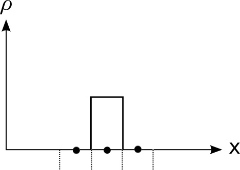
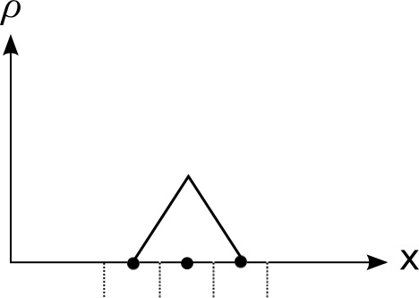
Various methods of mapping particles to a grid exist, depending on the amount of smoothing needed. The commonly used methods are Cloud-In-Cell (CIC) and Triangualr-Shaped-Cloud (TSC) assignment. Densfield supports both for dark matter type particles and uses TSC as a default. The weighting kernel of the two methods is shown below:

Kernel of the Cloud-In-Cell (CIC) assignment technique along one dimension. The smoothing length in this kernel is one cell. [JPG]

Kernel of the Triangular-Shaped-Cloud (TSC) assignment technique along one dimension. The smoothing length in this kernel is three cells. [JPG]

These kernels are then centered on the position of each particle and intersected with the target grid (we map quantities zonal, i.e. in regard to the cell center). In the case of CIC and TSC this is done analytically, however with the more elaborate SPH kernel mapping described below, a numerical approach is chosen.

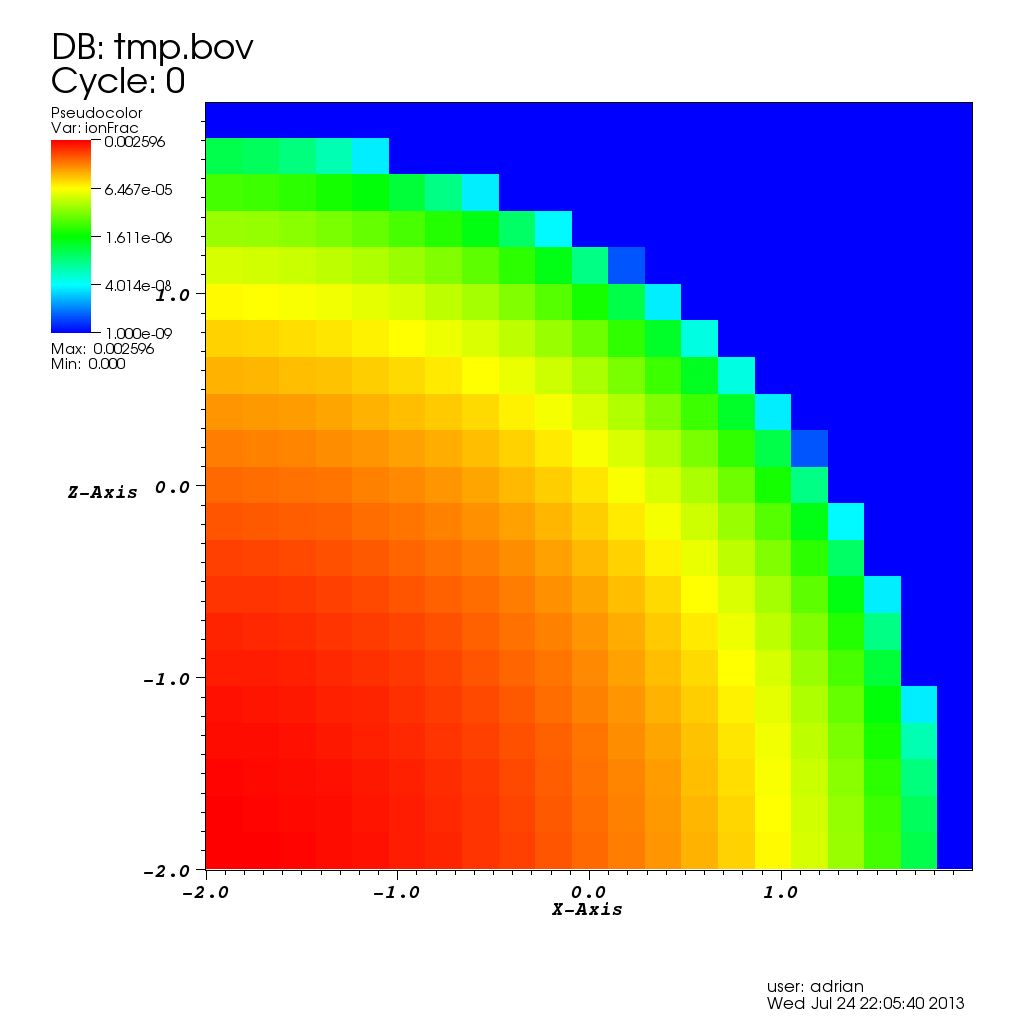
SPH Kernel Mapping

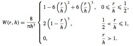
State of the art cosmological simulations also follow the evolution of gas. Gas can either be solved with mesh based techniques using Riemann solvers or with the Smoothed Particle Hydrodynamics (SPH) technique. With the widely used SPH method, the need for mapping particles onto a grid can arise again in the analysis of the simulations. This however is a non trivial task, since the SPH kernel used to describe each particle (in SPH a particle is not a point but more like an extended and compressible sphere) is complicated. The SPH kernel implemented in the widely used GADGED code and used by densfield has the following functional form (the radius r of the kernel is determined by a given number of nearest particles and is provided with the simulation output):

Some tools available on the internet claiming to map SPH particles onto a grid just evaluate the SPH kernel of each particle at the position of the cell and accumulate this value. This approach is easy and maybe useful for visualisation purposes, but is completely useless for scientific analysis. This becomes evident if one considers a particle with a radius a fraction of a grid cell. Evaluating the kernel at the cell position will result in the value 0, and thus does not contribute to the cell. However it should be fully accounted for. These codes thus loose mass (or whatever variable is mapped to the grid) and obtain wrong quantities.

In order to correctly map a SPH quantity onto a grid, one needs to integrate the SPH kernel over the extend of the cell. This is what densfield does. Only then, a correct mapping of the SPH smoothing information can be achieved (you can always use CIC or TSC as well, but this is not part of the exercise here).

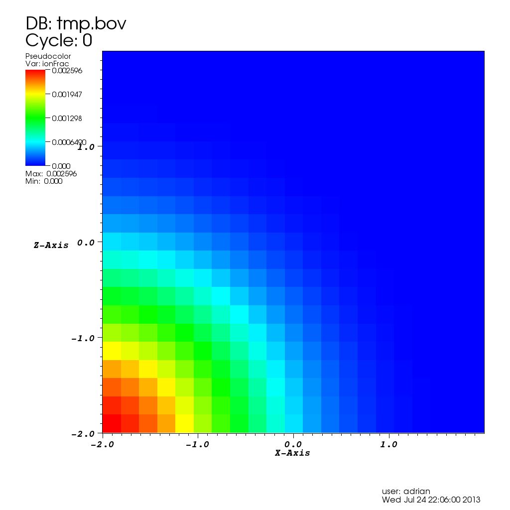
It is computationally unfeasible to integrate the SPH kernel for each particle over each intersected cell. In order to make this approach feasible, we precompute the SPH kernel in various grid sizes and fully integrate the kernel over the extend of each cell. An example of such a precomputed SPH kernel is given below:

The SPH Kernel in linear scale on a grid of 21×21 cells (Note: Kernel is normalised) [JPG]

The SPH Kernel in logarithmic scale on a grid of 21×21 cells, showing its vast extent (Note: Kernel is normalised) [JPG]

These precomputed SPH kernels are then centered on each particle position and then intersected with the target grid. Values in this process are assigned in a CIC fashion. Since the SPH kernel can have different radii and to reduce the number of calculations in the mapping, densfield uses 3 different resolutions of the precomputed SPH kernel in the assignment: Default values for grid sizes are SPHKERNELSIZESMALL: 3, SPHKERNELSIZEMEDIUM: 7, SPHKERNELSIZEBIG: 15. These values can be adjusted in the configuration file. Depending on the ratio of the SPH kernel radius to the target grid cell, the corresponding resolution is chosen in the assignment.

This approach enables a fast and quantity conserving tool for mapping SPH particles onto a grid.