PaQu: Parallel Queries for MySQL

Introduction

The tables in the MultiDark DB have reached sizes that are hard to query and manage using currently available single node databases. A solution that is widely used to overcome this problem are so called Hadoop Clusters. In Hadoop, data is chopped up into small pieces and distributed over many data nodes. When querying, the job is transmitted to all data nodes and the result is then sent back to the head node. This approach is rather popular and successful with companies like Google and Facebook. However the downside is, that a new query paradigm needs to be learned (the Map/Reduce paradigm) which is completely different to SQL and compares rather to parallel programming using MPI.

We therefore wanted to build on the idea of distributed data. However we want to retain the use of database systems and SQL as a query language. A couple of commercial products supporting distributed databases and distributed querying exist. Nevertheless we decided to push for an open source solution to promote the development of such open systems. Our choice fell on the MySQL Spider parallel storage engine to manage our data and the shard-query project. Shard-query relies on the Gearman job queue framework for achieving parallelisation. PaQu however was designed to solely rely on the MySQL Spider engine. We have extensively extended the shard-query tool to support SQL queries as they are needed by scientists. As a result, not much of shard-query was left and the new parallel query tool PaQu was born.

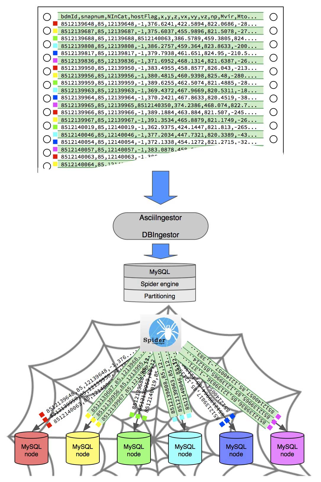
In the end, the general idea is to formulate solution from given SQL queries the “Map/Reduce” way. PaQu compares to Hive, which translates SQL queries into Map/Reduce jobs for Hadoop. Similar restrictions applying to Hive also apply to PaQu due to the nature of the problem. PaQu solely relies in the RDBMS world and uses plain SQL together with the MySQL Spider engine UDFs to perform the parallelisation. PaQu itself is written in PHP, due to the origins in the shard-query tool. The complete architecture of PaQu is given below:

At the new MultiDark database we have 10 dedicated database nodes that serve data to the user. This gives the user in the most optimal case a factor 10 times faster queries. However the speed up will be somewhat lower, due to communication overhead (data needs to be transferred to the head node and back to the database nodes, depending on how complex your queries are).

This document will describe how PaQu works from a more technical point of view (and will probably grow with time to describe more technical aspects), why it does what it does, and how it is used.

Since PaQu is still under heavy development, some bugs most surely still exist and we are happy to know of every query that does not yet work with PaQu. We have provided an easy way to submit erroneous queries from within the query form, as soon as the query plan is shown. Please make use of it so that we can improve PaQu! Thanks!

Distributed Tables

The first concept we need to get familiar with are distributed database tables. Up to now, all tables in the MultiDark database have been tables that resided as whole on one database node. A query would then go through the complete table (a so called full table scan) and retrieve the results. With distributed tables things are slightly different.

The database head node (running the Spider engine) will take the data in the table and chop it up into N pieces (in our case 10 tables for 10 database nodes). These tables are then sent to the respective database nodes and stored there. The rule with which the tables are chopped up can depend on the use case, however we have considered a universal use case and distributed the tables equally to the nodes.

This part of the process is still outside of PaQu and is solely achieved through the MySQL Spider engine. There, so called partitioned tables are created using MySQL native functionality. To each resulting partition a data node is assigned. The data is then ingested into the head node using our DBIngestor library or our AsciiIngest tool (which is build using the DBIngestor library) and the MySQL Spider engine takes care of the distribution of the data to each nodes, according to the chosen partitioning strategy. Since our intention was to speed up full table scans, we distribute the data as evenly amongst the data nodes as possible.

This concept is illustrated below:

If a user now wants to retrieve data from the distributed table, a query is sent to the head node, the head node will pass the query to each database node using the MySQL Spider UDF spider_bg_direct_sql and the nodes search the table for the desired data in parallel. After the data is found, the results are sent to the head node and made available to the user. The results are returned to the head node through tables that are residing on the head node and are linked to the data nodes using the Federated storage engine. This is the actual bottle neck of PaQu, since locking issues arise when all the data nodes write back their results (we are using MyISAM for performance and there table locks are used).

In principle, the procedure is equal to the one in the undistributed case, especially in the case of simple queries. Things start to look different if the results of table A need to be combined with table B. In these cases, the SQL query cannot be simply passed on to each node and processed there. It might be, that node 1 needs to combine data that lies on node 2. This is where it becomes tricky and PaQu helps you as much as possible.

PaQu will analyse your query, first ask all nodes for the information in table A that needs to be combined with table B and gathers it on the head node. Then the result of this sub-query is passed back to all the nodes and can then be combined with table B. PaQu thus tries to parallelise these so called JOINs. Since PaQu (contrary to Hive) does not store any statistics of the tables yet, PaQu relies on a crude heuristic to choose which table to ask first for results. In theory, to reduce the amount of falsely queries data, this would be the table that has the highest selectivity. However PaQu does not know the selectivity and will ask the table with the most independent restrictions given with the WHERE clause first. This does not need to be the most optimal choice but has proven to work quite well up to now.

How PaQu works is discussed in more detail below.

What is PaQu and What are Parallel Queries?

PaQu, the parallel query facility, is a tool that takes an input SQL query and transforms it into a parallel one running on a MySQL Spider engine cluster. This involves the analysis of the query, finding of JOINs (implicit and explicit), finding of aggregate functions (COUNT, AVG, STDEV…) and the production of a parallel query execution plan.

PaQu takes the SQL query and analyses it to create a so called parse tree; a tree of all the SQL commands in the query retaining any hierarchies introduced by sub-queries. This parse tree is then traversed to find all aggregate functions, implicit JOINs (there are JOIN of the type SELECT a.*, b.* FROM a, b WHERE a.id = b.id) and register all sub-queries (SELECT a.* FROM a, (SELECT * FROM b) as b WHERE b.z = (SELECT z FROM redshifts WHERE snapnum=85)). The parse tree is then processed and restructured according to rules briefly explained throughout this document. After a new parse tree is obtained, it is transformed into a parallel query plan, that can be executed by PaQu on the MySQL head node.

At this stage, PaQu has reformulated all JOINs into sub-queries that can be run successively according to relational algebra (using the simplistic heuristic described above) and has reformulated all aggregate functions into their appropriate parallel counter parts (COUNT -> SUM, AVG -> SUM / COUNT, STDEV -> Welford Algorihm UDFs (see Online Variance algorithms on Wikipedia for more information). The parallel query plan will inform you, which sub-query is run first, in which temporary tables results are saved and how they are further combined into the final result table.

In the process of restructuring, column names are aliased to unique names and great care is given to preserve given aliases as much as possible. However since the query is completely restructured into a set of nested sub-queries, this is not always possible. However in the final reduction step, the column names are transformed back into what the user would expect.

Since PaQu is still in Beta stage and needs further hardening, the query plan is presented to the user in the new MultiDark interface. The user can follow what PaQu does and evaluate if this is the correct way of parallelising the query or not. If not, a possibility is given to alter the parallel query plan manually and submit the query for bug-fixing to the PaQu developers (if Daiquiri is used).

In order to understand in more detail how the parallel query plan is read, let’s discuss the three basic operations used in parallelising queries and illustrate the concept using simple examples.

How to Read and Modify the Parallel Query Plan

After the SQL query is analysed and optimised for parallel execution, a parallel query plan which governs the parallel execution of the query is generated. The parallel query plan is valid SQL using “pseudo-UDFs” functions (pseudo, because PaQu needs to convert them to a complex set of SQL queries). The three functions governing all parallelisation tasks are:

• paquExec
• paquLinkTmp
• paquDropTmp

Any other reduction tasks are completely implemented in SQL and are also part of the parallel query plan.

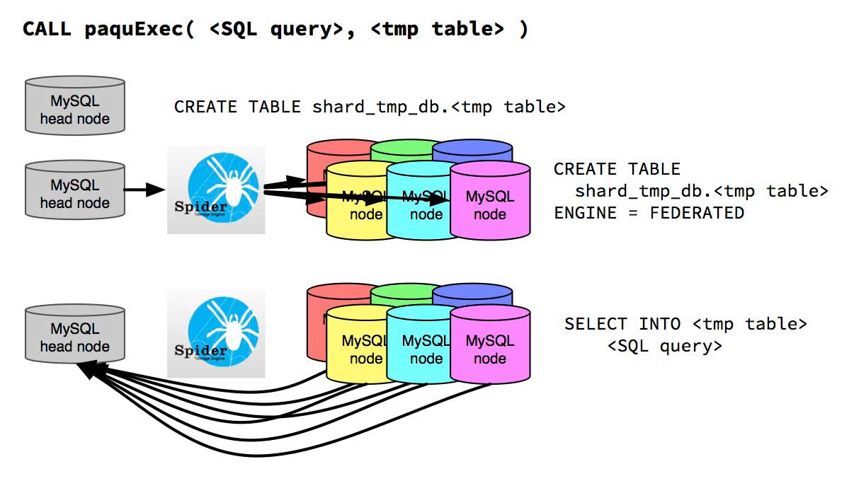
paquExec( < SQL query >, < tmp table > )

paquExec executes the SQL statement given in <SQL query> on each node. They are executed as is and are not transformed any further (this is not quite true, since the name of the destination temporary table is added to the query). Before paquExec executes the query, a temporary data table <tmp table> is created in the PaQu scratch table database. This temporary table resides on the head node and is shared with all data nodes. The sharing is achieved by creating Federated tables on all data nodes pointing to the temporary table on the head node. The results of the are locally (on each node) inserted into `` and are transferred to the head node using MySQL (this is automatically achieved through the Federated engine). It is good to keep in mind, that this transfer poses the biggest bottle neck in PaQu.

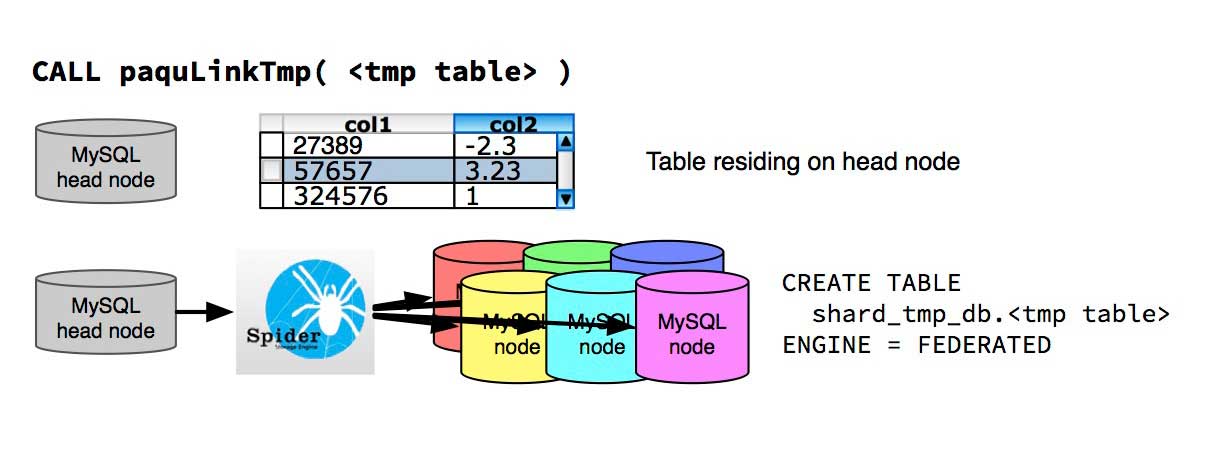
paquLinkTmp( < tmp table > )

paquLinkTmp links a table <tmp table> that completely resides on the head node (this could be the result of a previous query) with the data nodes. NOTE: In order to use this function, data needs to be copied into the PaQu scratch database first – into <tmp table>! This is needed since PaQu itself should only have access to the scratch database for various reasons. The simplest reason however is, that by dropping and recreating the scratch database, any remaining Federated table that might hang out in the wild can be easily destroyed. Eventually, the temporary table becomes available on the data nodes and can be used in JOINs with the distributed data.

paquDropTmp( < tmp table > )

paquDropTmp will drop a temporary table <tmp table> in the PaQu scratch database on the data nodes (removing the Federated links) and then on the head node (removing the actual data).

Examples

The concept of how the parallelisation works will be explained with the following two examples. One example will show how the parallel query plan of aggregation queries looks like, and the second example will involve an implicit join.

Aggregation

The following query would calculate the mean mass and corresponding standard deviation for each snapshot in the FOF table of the MDR1 database:

SELECT snapnum, avg(mass), stddev(mass) FROM MDR1.FOF GROUP BY snapnum;

The corresponding query plan would look like:

CALL paquExec("SELECT snapnum AS `snapnum`, COUNT(mass) AS `cnt_avg(mass)`, SUM(mass) AS `sum_avg(mass)`, sum_of_squares(mass) AS `ssqr_stddev(mass)`, AVG(mass) as `avg_stddev(mass)`, COUNT(mass) AS `cnt_stddev(mass)` FROM MDR1.FOF GROUP BY snapnum ORDER BY NULL ", "aggregation_tmp_8896713");
USE spider_tmp_shard; SET @i=0; CREATE TABLE multidark_user_admin.`/*@GEN_RES_TABLE_HERE*/` ENGINE=MyISAM SELECT DISTINCT @i:=@i+1 AS `row_id`, `snapnum`, (SUM(`sum_avg(mass)`) / SUM(`cnt_avg(mass)`)) AS `avg(mass)`, SQRT(partitAdd_sum_of_squares(`ssqr_stddev(mass)`, `avg_stddev(mass)`, `cnt_stddev(mass)`) / (SUM(`cnt_stddev(mass)`) - 1)) AS `stddev(mass)`
FROM `aggregation_tmp_8896713` GROUP BY `snapnum` ;
CALL paquDropTmp("aggregation_tmp_8896713");

The first line in the query plan, involves a paquExec call, which executes the contained SQL statement on all nodes and writes back the result in the temporary table aggregation_tmp_8896713:

CALL paquExec("SELECT snapnum AS `snapnum`, COUNT(mass) AS `cnt_avg(mass)`, SUM(mass) AS `sum_avg(mass)`, sum_of_squares(mass) AS `ssqr_stddev(mass)`, AVG(mass) as `avg_stddev(mass)`, COUNT(mass) AS `cnt_stddev(mass)` FROM MDR1.FOF GROUP BY snapnum ORDER BY NULL ", "aggregation_tmp_8896713");

As can be seen, the AVG function in transformed into a COUNT and SUM statement, and the STDDEV statement into the sum_of_squares, AVG, and COUNT function for the Welford Algorihm. The results are GROUP BYed on each node on its own and separately combined later.

The second query would be a reduction query run on the head node to combine all the results of the different nodes:

USE spider_tmp_shard; SET @i=0; CREATE TABLE multidark_user_admin.`/*@GEN_RES_TABLE_HERE*/` ENGINE=MyISAM SELECT DISTINCT @i:=@i+1 AS `row_id`, `snapnum`, (SUM(`sum_avg(mass)`) / SUM(`cnt_avg(mass)`)) AS `avg(mass)`, SQRT(partitAdd_sum_of_squares(`ssqr_stddev(mass)`, `avg_stddev(mass)`, `cnt_stddev(mass)`) / (SUM(`cnt_stddev(mass)`) - 1)) AS `stddev(mass)` FROM `aggregation_tmp_8896713` GROUP BY `snapnum` ;

The database is changed to spider_tmp_shard using

USE spider_tmp_shard;

and a variable for counting the lines in the result table is set to zero

SET @i=0;

Then the result table is created on the user database side with the name of the table being inserted later at execution time. However a placeholder for the table name /*@GEN_RES_TABLE_HERE*/ marks where the name will be inserted. Then follows the reduction query combining the results and adding a row number column as the first column:

CREATE TABLE multidark_user_admin.`/*@GEN_RES_TABLE_HERE*/` ENGINE=MyISAM SELECT DISTINCT @i:=@i+1 AS `row_id`, `snapnum`, (SUM(`sum_avg(mass)`) / SUM(`cnt_avg(mass)`)) AS `avg(mass)`, SQRT(partitAdd_sum_of_squares(`ssqr_stddev(mass)`, `avg_stddev(mass)`, `cnt_stddev(mass)`) / (SUM(`cnt_stddev(mass)`) - 1)) AS `stddev(mass)` FROM `aggregation_tmp_8896713` GROUP BY `snapnum` ;

It can be seen, that the AVG is being reduced by the SUM of the sum of all masses on the individual nodes, divided by the SUM of all the number of rows contributing to the sum of all masses on the individual nodes. The STDDEV is combined according to the Welford Algorithm using a partitioned addition of all the sum of squares divided by the SUM of all the number of rows contributing to the STDDEV of the masses on the individual nodes. Again, the results is GROUP BYed on the reduction query in order to retain the different bins and only apply the reduction step individually to each bin.

CALL paquDropTmp("aggregation_tmp_8896713");

As a remaining step, the temporary table aggregation_tmp_8896713 is destroyed using paquDropTmp on the head and compute nodes.

Implicit Join

The following query would get for all FOF haloes the corresponding particles (limiting the result only to 10 particles).

SELECT `part`.* from MDR1.FOFParticles AS `part`, MDR1.FOF AS `hal` WHERE FOFParticles.fofId=FOF.fofId LIMIT 10;

Paqu will identify the implicit join in the query and split it into two sub-queries. The corresponding query plan would look like:

CALL paquExec("SELECT `part`.fofParticleId  AS `part__fofParticleId`,`part`.fofId  AS `part__fofId`,`part`.particleId  AS `part__particleId`,`part`.snapnum  AS `part__snapnum` FROM MDR1.FOFParticles AS `part` ORDER BY NULL  LIMIT 0,10", "aggregation_tmp_52267557");
CALL paquExec("SELECT `part`.`part__fofParticleId` AS `part__fofParticleId`,`part`.`part__fofId` AS `part__fofId`,`part`.`part__particleId` AS `part__particleId`,`part`.`part__snapnum` AS `part__snapnum` FROM MDR1.FOF AS `hal` JOIN ( SELECT `part__fofParticleId`,`part__fofId`,`part__particleId`,`part__snapnum` FROM `aggregation_tmp_52267557`    LIMIT 0,10) AS `part`  WHERE (  `part`.`part__fofId` = `hal`.fofId )   ", "aggregation_tmp_54927163");
CALL paquDropTmp("aggregation_tmp_52267557");
USE spider_tmp_shard; SET @i=0; CREATE TABLE multidark_user_adrian.`/*@GEN_RES_TABLE_HERE*/` ENGINE=MyISAM SELECT DISTINCT @i:=@i+1 AS `row_id`,  `part__fofParticleId`,`part__fofId`,`part__particleId`,`part__snapnum`
FROM `aggregation_tmp_54927163`   ;
CALL paquDropTmp("aggregation_tmp_54927163");

The first line in the query plan, involves a paquExec call, which executes the contained SQL statement on all nodes and writes back the result in the temporary table aggregation_tmp_52267557:

CALL paquExec("SELECT `part`.fofParticleId  AS `part__fofParticleId`,`part`.fofId  AS `part__fofId`,`part`.particleId  AS `part__particleId`,`part`.snapnum  AS `part__snapnum` FROM MDR1.FOFParticles AS `part` ORDER BY NULL  LIMIT 0,10", "aggregation_tmp_52267557");

Paqu has identified the FOFParticles table to be the first table that will be queried. In this query, both tables have equal priority and the query does not imply that one table is more important than the other. Since a LIMIT clause is added to the query, the LIMIT clause will be pushed down to the sub-query. Since only 10 rows are asked for, it does not make sense to retrieve the whole FOFParticles table to the head node. A smaller subset already fulfills the query.

After some rows of FOFParticles are returned to the head node (exactly number_of_nodes * number_of_requested_rows), the second query will carry out the implicit join with the FOF table:

CALL paquExec("SELECT `part`.`part__fofParticleId` AS `part__fofParticleId`,`part`.`part__fofId` AS `part__fofId`,`part`.`part__particleId` AS `part__particleId`,`part`.`part__snapnum` AS `part__snapnum` FROM MDR1.FOF AS `hal` JOIN ( SELECT `part__fofParticleId`,`part__fofId`,`part__particleId`,`part__snapnum` FROM `aggregation_tmp_52267557`    LIMIT 0,10) AS `part`  WHERE (  `part`.`part__fofId` = `hal`.fofId )   ", "aggregation_tmp_54927163");

At this stage, the table aggregation_tmp_52267557 is already shared with all the nodes and the FOFParticles data from the various node collected on the head node is made available to all nodes for the JOIN. The JOIN with the FOF table is executed on each node and the results are sent back to the head node into table aggregation_tmp_54927163. Note, the LIMIT clause is again applied in the JOIN step, since a small subset of the result set already fulfills the query.

Afterwards the temporary table aggregation_tmp_52267557 is destroyed, since it is not needed anymore:

CALL paquDropTmp("aggregation_tmp_52267557");

And the result is reduced/written to the final result table. Again, the LIMIT clause is added to the reduction query to finally reduce the result set to the requested length:

USE spider_tmp_shard; SET @i=0; CREATE TABLE multidark_user_adrian.`/*@GEN_RES_TABLE_HERE*/` ENGINE=MyISAM SELECT DISTINCT @i:=@i+1 AS `row_id`,  `part__fofParticleId`,`part__fofId`,`part__particleId`,`part__snapnum`
FROM `aggregation_tmp_54927163`   ;

The final cleanup requires the deletion of the aggregation_tmp_54927163 temporary table:

CALL paquDropTmp("aggregation_tmp_54927163");